本文由医信融合团队成员“陈浩然”撰写,已同步至微信公众号“医信融合创新沙龙”与“研究生学生信”,更多精彩内容欢迎关注!


在之前的推送中,介绍了通路的激活与抑制关系(如何判断你的信号通路已经激活**?**),而在研究转录组数据时,筛选出差异基因后,如果能够预测并理清基因之间的调控关系,对于后续的实验、临床研究也有一定的帮助。
CBNplot 以富集分析结果为基础,利用贝叶斯网络图通过分析富集通路以及通路中基因之间的关系,推断基因调控网络,促进从基因表达谱中挖掘出更多有用的数据。
0
分析之前准备工作
首先需要安装相关的包,配置相关环境。为什么要配置环境,可以参考之前的文章([KEGG 数据库报错及解决](http://mp.weixin.qq.com/s?__biz=Mzk0MDI4MjM4NQ==&mid=2247483814&idx=1&sn=0e7124c06a5a7c690ab824f84a60fc08&chksm=c2e546d8f592cfce8ca0841aa96c20c120e8c1be12e51754772593f8c8e8d4695deee52ac97c&scene=21#wechat_redirect))
#####
#0.Before analysis
#####
# Import the package
library("clusterProfiler")
library("DESeq2")
library("ggplot2")
library("ReactomePA")
library("CBNplot")
# Environment setting
getOption("clusterProfiler.download.method")
R.utils::setOption( "clusterProfiler.download.method",'auto')
Sys.setlocale(category = "LC_ALL",locale = "English_United States.1252")
1
差异分析
这一步是以 GEO 中 GSE133624 的 supplementary file 为例,使用 DEseq2 算法进行差异分析。不同的数据需要选择不同的分析算法,可以参考四文搞定 GEO 数据库转录组差异分析之操作。其中,第 5 行的工作路径需要自行修改
#####
#1.Differential expression analysis
#####
# Set the working directory
setwd("C:\\Users\\13415\\Desktop\\GRN")
## Load dataset and make metadata
counts = read.table("GSE133624_reads-count-all-sample.txt.gz", header=1, row.names=1)
meta = sapply(colnames(counts), function (x) substring(x,1,1))
meta = data.frame(meta)
colnames(meta) = c("Condition")
dds <- DESeqDataSetFromMatrix(countData = counts,
colData = meta,
design= ~ Condition)
## Prefiltering
filt <- rowSums(counts(dds) < 10) > dim(meta)[1]*0.9
dds <- dds[!filt,]
## Perform DESeq2()
dds = DESeq(dds)
res = results(dds, pAdjustMethod = "bonferroni")
## apply variance stabilizing transformation
v = vst(dds, blind=FALSE)
vsted = assay(v)
## Plot PCA of VST values
DESeq2::plotPCA(v, intgroup="Condition")+
theme_bw()
2
富集分析
#####
#2.Enriment analysis
#####
## Define the input genes, and use clusterProfiler::bitr to convert the ID.
sig = subset(res, padj<0.05)
ensembl_entrez = bitr(rownames(sig), fromType="ENSEMBL", toType="ENTREZID", OrgDb=org.Hs.eg.db)
cand.entrez = symbol_entrez$ENTREZID
## Perform enrichment analysis (ORA)
pway = enrichPathway(gene = cand.entrez,readable = T)
pwayGO = enrichGO(cand.entrez, ont = "BP", OrgDb = org.Hs.eg.db,readable = T)
## Store the similarity
pway = enrichplot::pairwise_termsim(pway)
## Define including tumor samples
incSample = rownames(subset(meta, Condition=="T"))
## enriment plot
barplot(pway, showCategory = 10)
3
一行代码简单查看一下基因间关系
#####
# 3. Gene regulatory network plot
#####
bngeneplot(results = pway, exp = vsted[,incSample], pathNum = 17)
点的大小和颜色代表基因的表达量,线的粗细、颜色代表关联强度,但是分析其实还有很多花样的,因为这个函数的参数有几十个
 ,而且吧,这个描述比较模糊,需要一个一个尝试。
4
调整一些参数试试
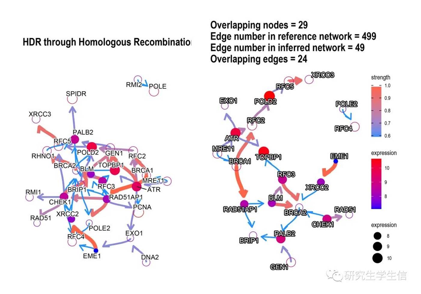
设置 compareRef=TRUE,可以查看参考网络,参考网络为已经证实的网络。
#####
#4. Pathway regulatory network plot
#####
cl = makeCluster(4)
GRN_plot<-bngeneplot(results = pway,
exp = vsted,
expSample = incSample,
pathNum = 17, R = 10, compareRef = T,
convertSymbol = T, pathDb = "reactome",
expRow = "ENSEMBL", cl = cl)
ggsave(GRN_plot, filename = "gene_regulatory_plot.PDF", device = cairo_pdf,
width = 10, height = 7, units = "in")
设置 hub=10,可以展示 top10 的关键基因(实心点)
#####
#5. Pathway regulatory network plot with 10 hub gene
#####
GRN_REF_plot<-bngeneplot(results = pway,
exp = vsted,
expSample = incSample,
pathNum = 17, R = 10, compareRef = T,
convertSymbol = T, pathDb = "reactome",
expRow = "ENSEMBL", cl = cl,hub = 10)
ggsave(GRN_REF_plot, filename = "gene_regulatory_REF_plot.PDF", device = cairo_pdf,
width = 10, height = 7, units = "in")
stopCluster(cl) # close the cluster
参数实在太多了,感觉一天学不完了,下期有机会,把这几十个参数一一搞定。同时还挖一个坑,就是通路间的上下游调控关系,也能做出来!


忙活一天,小赚 20
同时,公众号对话窗口回复基因调控,即可免费领取输入文件、代码、输出结果,结果以 Rproject 格式打包,想要了解如何使用 Rproject 可以参考3.GEO 的 ID 转换已经通关了,Ctrl+A、然后 Ctrl+Enter,即可获得本文的全部结果

感谢您观看到最后,敬请批评指正!
图文:陈浩然
本文编辑:李晨龙