本文由医信融合团队成员“张皓旻”撰写，已同步至微信公众号“医信融合创新沙龙”，更多精彩内容欢迎关注！

转录组测序的目的之一，就是探索组间显著表达变化的基因——差异表达基因。那么，如何基于转录组测序获得的定量表达值，识别差异表达变化的基因或其它非编码RNA分子呢？DESeq2是目前文献中寻找差异基因使用频率最高的R包之一。本文测试数据使用GSE176393。

DESeq2安装：

DESeq2的安装很简单，直接在R语言中使用bioconduct进行安装即可。

#若未安装“BiocManager”
if (!require("BiocManager", quietly = TRUE))
install.packages("BiocManager")
BiocManager::install("DESeq2")
#若已安装“BiocManager”
library(BiocManager)
BiocManager::install("DESeq2")

安装完成直接library使用即可。

library(DESeq2)
载入需要的程辑包：S4Vectors
载入需要的程辑包：stats4
载入需要的程辑包：BiocGenerics
载入程辑包：‘BiocGenerics’
The following objects are masked from ‘package:stats’:
IQR, mad, sd, var, xtabs
The following objects are masked from ‘package:base’:
anyDuplicated, append, as.data.frame, basename, cbind, colnames, dirname, do.call, duplicated, eval, evalq,
Filter, Find, get, grep, grepl, intersect, is.unsorted, lapply, Map, mapply, match, mget, order, paste, pmax,
pmax.int, pmin, pmin.int, Position, rank, rbind, Reduce, rownames, sapply, setdiff, sort, table, tapply, union,
unique, unsplit, which.max, which.min
载入程辑包：‘S4Vectors’
The following objects are masked from ‘package:base’:
expand.grid, I, unname
载入需要的程辑包：IRanges
载入程辑包：‘IRanges’
The following object is masked from ‘package:grDevices’:
windows
载入需要的程辑包：GenomicRanges
载入需要的程辑包：GenomeInfoDb
载入需要的程辑包：SummarizedExperiment
载入需要的程辑包：MatrixGenerics
载入需要的程辑包：matrixStats
载入程辑包：‘MatrixGenerics’
The following objects are masked from ‘package:matrixStats’:
colAlls, colAnyNAs, colAnys, colAvgsPerRowSet, colCollapse, colCounts, colCummaxs, colCummins, colCumprods,
colCumsums, colDiffs, colIQRDiffs, colIQRs, colLogSumExps, colMadDiffs, colMads, colMaxs, colMeans2, colMedians,
colMins, colOrderStats, colProds, colQuantiles, colRanges, colRanks, colSdDiffs, colSds, colSums2, colTabulates,
colVarDiffs, colVars, colWeightedMads, colWeightedMeans, colWeightedMedians, colWeightedSds, colWeightedVars,
rowAlls, rowAnyNAs, rowAnys, rowAvgsPerColSet, rowCollapse, rowCounts, rowCummaxs, rowCummins, rowCumprods,
rowCumsums, rowDiffs, rowIQRDiffs, rowIQRs, rowLogSumExps, rowMadDiffs, rowMads, rowMaxs, rowMeans2, rowMedians,
rowMins, rowOrderStats, rowProds, rowQuantiles, rowRanges, rowRanks, rowSdDiffs, rowSds, rowSums2, rowTabulates,
rowVarDiffs, rowVars, rowWeightedMads, rowWeightedMeans, rowWeightedMedians, rowWeightedSds, rowWeightedVars
载入需要的程辑包：Biobase
Welcome to Bioconductor
Vignettes contain introductory material; view with 'browseVignettes()'. To cite Bioconductor, see
'citation("Biobase")', and for packages 'citation("pkgname")'.
载入程辑包：‘Biobase’
The following object is masked from ‘package:MatrixGenerics’:
rowMedians
The following objects are masked from ‘package:matrixStats’:
anyMissing, rowMedians

差异分析过程

DESeq2是一种基于负二项式分布的方法，使用局部回归推算均值和方差，通过离散度和倍数变化的收缩率估计以提高稳定性。定量分析关注的更多是差异表达的“强度”，而非“存在”。

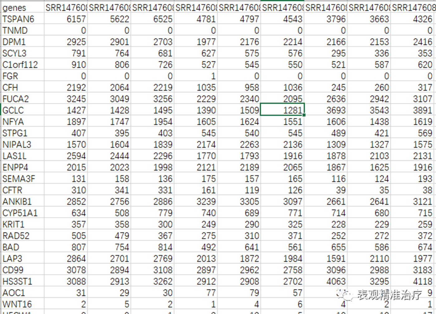
输入数据准备

表达量矩阵（我们就是用之前使用HTSeq定量的结果即可），若有自己的数据要求如下：

• 输入数据是由整数组成的矩阵。

• 矩阵是没有标准化的。

差异分析

===========

DESeq2包分析差异表达基因简单来说只有三步：构建dds矩阵，标准化，以及进行差异分析，我利用以下代码实现：

setwd("F:/RNA-Seq/GSE176393（SRP323246）/5-Diff")
library(DESeq2)
#读入输入数据，设计差异分组
rawdata <- read.table("rawread.txt",header=T,sep = "\t",row.names = 1)
diffcount <- rawdata[,1:6] ##由于我的数据有三个条件，所以我把需要进行差异分析的两组数据挑选出来，若分析数据仅包含两种条件则可不运行
sampleTable <- data.frame(condition = factor(rep(c("Control", "shBmal1"), each = 3))) ##可以依据实际情况修改各个条件的名称及数量
#构建dds矩阵
dds <- DESeqDataSetFromMatrix(countData = round(diffcount), colData = sampleTable, design = ~condition)
#对原始dds进行normalize
dds <- DESeq(dds)
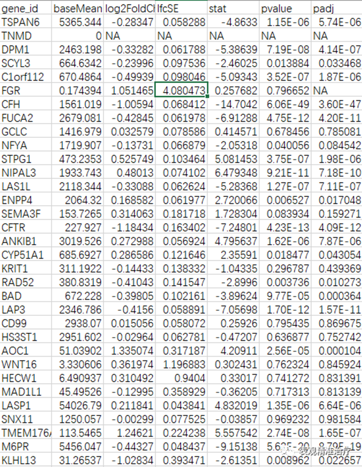
res <- results(dds)#将结果用results()函数来获取，赋值给res变量
#保存全部差异结果
diff_res <- as.data.frame(res)
diff_res$gene_id <- rownames(diff_res)
diff_res<-diff_res[, colnames(diff_res)[c(7,1:6)]]
write.table(diff_res,file = 'All_DESeq2_results.xls',sep = '\t',row.names = FALSE)
#依据提取符合阈值的差异结果
table(diff_res$padj<0.05) #取FDR小于0.05的结果，阈值可依据实际需要调整
diff_FDR <- diff_res[order(diff_res$padj),]
diff_gene_deseq2_FDR <-subset(diff_FDR,padj < 0.05 & (log2FoldChange > 1 | log2FoldChange < -1)) #阈值可依据实际需要调整
write.table(diff_gene_deseq2_FDR,file= "diff_gene_deseq2_FDR.xls",sep = '\t',row.names = F)
table(diff_res$pvalue<0.05) #取P值小于0.05的结果
diff_p <- diff_res[order(diff_res$pvalue),]
diff_gene_deseq2_p <-subset(diff_p,pvalue < 0.05 & (log2FoldChange > 1 | log2FoldChange < -1)) #阈值可依据实际需要调整
write.table(diff_gene_deseq2_p,file= "diff_gene_deseq2_pvalue.xls",sep = '\t',row.names = F)

结果如下图：

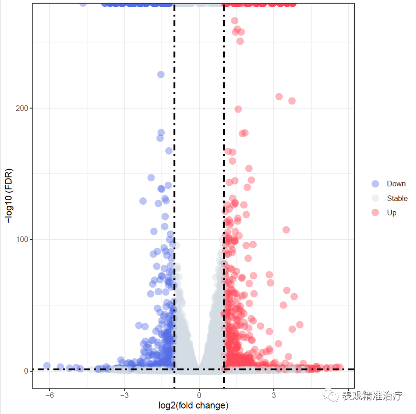
结果可视化

差异结果的可视化以火山图形式呈现：

#绘制火山图(FDR筛选)
library(ggplot2)
cut_off_stat = 0.05 #设置统计值阈值
cut_off_logFC = 1 #设置表达量阈值,可修改
diff_res[is.na(diff_res)] <- 0
diff_res$change = ifelse(diff_res$padj < cut_off_stat & abs(diff_res$log2FoldChange) >= cut_off_logFC,
ifelse(diff_res$log2FoldChange> cut_off_logFC ,'Up','Down'),
'Stable')
pdf("volcanol_FDR.pdf")
ggplot(diff_res,
aes(x = log2FoldChange,
y = -log10(padj),
colour=change)) +
geom_point(alpha=0.4, size=3.5) +
scale_color_manual(values=c("#546de5", "#d2dae2","#ff4757"))+
geom_vline(xintercept=c(-1,1),lty=4,col="black",lwd=0.8) +
geom_hline(yintercept = -log10(cut_off_stat),lty=4,col="black",lwd=0.8) +
labs(x="log2(fold change)",
y="-log10 (FDR)")+
theme_bw()+
theme(plot.title = element_text(hjust = 0.5),
legend.position="right",
legend.title = element_blank()
)
dev.off()
#绘制火山图(pvalue筛选)
library(ggplot2)
cut_off_stat = 0.05 #设置统计值阈值
cut_off_logFC = 1 #设置表达量阈值,可修改
diff_res[is.na(diff_res)] <- 0
diff_res$change = ifelse(diff_res$pvalue < cut_off_stat & abs(diff_res$log2FoldChange) >= cut_off_logFC,
ifelse(diff_res$log2FoldChange> cut_off_logFC ,'Up','Down'),
'Stable')
pdf("volcanol_pvalue.pdf")
ggplot(diff_res,
aes(x = log2FoldChange,
y = -log10(pvalue),
colour=change)) +
geom_point(alpha=0.4, size=3.5) +
scale_color_manual(values=c("#546de5", "#d2dae2","#ff4757"))+
geom_vline(xintercept=c(-1,1),lty=4,col="black",lwd=0.8) +
geom_hline(yintercept = -log10(cut_off_stat),lty=4,col="black",lwd=0.8) +
labs(x="log2(fold change)",
y="-log10 (p-value)")+
theme_bw()+
theme(plot.title = element_text(hjust = 0.5),
legend.position="right",
legend.title = element_blank()
)
dev.off()
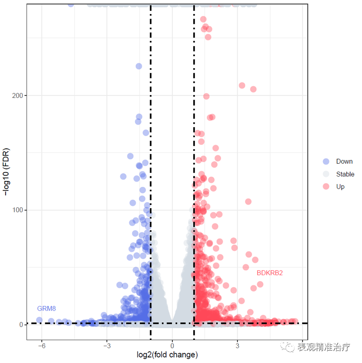
##绘制带有基因名称的火山图
library(ggplot2)
library(ggrepel)
cut_off_stat = 0.05 #设置统计值阈值
cut_off_logFC = 1 #设置表达量阈值,可修改
diff_res[is.na(diff_res)] <- 0
diff_res$change = ifelse(diff_res$pvalue < cut_off_stat & abs(diff_res$log2FoldChange) >= cut_off_logFC,
ifelse(diff_res$log2FoldChange> cut_off_logFC ,'Up','Down'),
'Stable')
diff_res$label = ifelse(diff_res$padj < cut_off_stat & abs(diff_res$log2FoldChange) >= 4, as.character(diff_res$gene_id),"")
pdf("volcanol_gene.pdf")
ggplot(diff_res,
aes(x = log2FoldChange,
y = -log10(padj),
colour=change)) +
geom_point(alpha=0.4, size=3.5) +
scale_color_manual(values=c("#546de5", "#d2dae2","#ff4757"))+
geom_vline(xintercept=c(-1,1),lty=4,col="black",lwd=0.8) +
geom_hline(yintercept = -log10(cut_off_stat),lty=4,col="black",lwd=0.8) +
labs(x="log2(fold change)",
y="-log10 (FDR)")+
theme_bw()+
theme(plot.title = element_text(hjust = 0.5),
legend.position="right",
legend.title = element_blank()
)+
geom_text_repel(data = diff_res, aes(x = diff_res$log2FoldChange,
y = -log10(diff_res$padj),
label = label),
size = 3,box.padding = unit(0.8, "lines"),
point.padding = unit(0.8, "lines"),
show.legend = FALSE)
dev.off()

获得如下结果：

图文：张皓旻

本文编辑：李新龙