本文由医信融合团队成员“张皓旻”撰写,已同步至微信公众号“医信融合创新沙龙”,更多精彩内容欢迎关注!

差异分析之后,为了了解我们获取的差异基因的功能及参与的生物学进程,我们需要对差异基因进行功能富集分析。实现富集分析的方法有很多,有许多数据库都可以进行,比如DAVID、KOBAS、Metascape等。今天我们先学习如何使用R语言中的clusterProfiler进行功能富集分析。
基因富集分析(gene set enrichment analysis)是在一组基因或蛋白中找到一类过表达的基因或蛋白。研究方法可分为三种:Over-Repressentation Analysis(ORA),Functional Class Scoring(FCS)和Pathway Topology。ORA是目前应用最多的方法,GO富集分析和KEGG富集分析就是使用的这种方法;FCS这种方法应用于GSEA分析。
功能分析(functional analysis)/通路分析(pathway analysis)是将一堆基因按照基因的功能/通路来进行分类。换句话说,就是把一个基因列表中,具有相似功能的基因放到一起,并和生物学表型关联起来。GO分析是将基因分门别类放入一个个功能类群,而pathway则是将基因一个个具体放到代谢网络中的指定位置。
为了解决将基因按照功能进行分类的问题,科学家们开发了很多基因功能注释数据库。这其中比较有名的就是Gene Ontology(基因本体论,GO)和Kyoto Encyclopedia of Genes and Genomes(京都基因与基因组百科全书,KEGG)。
clusterProfiler安装:
if (!require("BiocManager", quietly = TRUE))
install.packages("BiocManager")
BiocManager::install("clusterProfiler")
安装完成直接library使用即可。
library("clusterProfiler")
clusterProfiler v4.2.1 For help: https://yulab-smu.top/biomedical-knowledge-mining-book/
If you use clusterProfiler in published research, please cite:
T Wu, E Hu, S Xu, M Chen, P Guo, Z Dai, T Feng, L Zhou, W Tang, L Zhan, X Fu, S Liu, X Bo, and G Yu. clusterProfiler 4.0: A universal enrichment tool for interpreting omics data. The Innovation. 2021, 2(3):100141
载入程辑包:‘clusterProfiler’
The following object is masked from ‘package:stats’:
filter
富集分析
输入数据准备
KEGG富集
library("clusterProfiler")
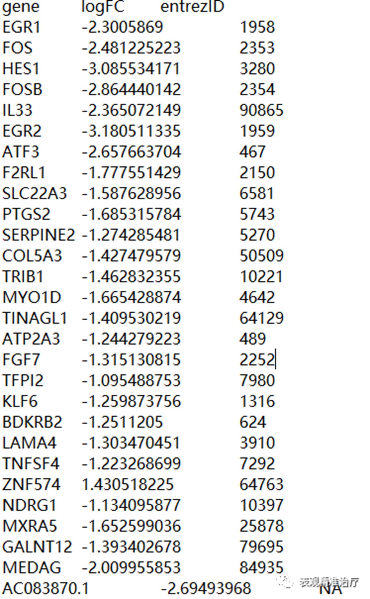
rt=read.table("id.txt",sep="\t",header=T,check.names=F)
rt=rt[is.na(rt[,"entrezID"])==F,]
geneFC=rt$logFC
gene=rt$entrezID
names(geneFC)=gene
#kegg富集分析
kk <- enrichKEGG(gene = gene, organism = "hsa", pvalueCutoff = 2, qvalueCutoff = 2)
write.table(kk,file="KEGG.txt",sep="\t",quote=F,row.names = F)
#条形图
tiff(file="barplot.tiff",width = 25,height = 25,units ="cm",compression="lzw",bg="white",res=300)
barplot(kk, drop = TRUE, showCategory = 20, main="30min")
dev.off()
#点图
tiff(file="dotplot.tiff",width = 27,height = 25,units ="cm",compression="lzw",bg="white",res=300)
dotplot(kk)
dev.off()
#绘制通路图
library("pathview")
keggxls=read.table("chosen.txt",sep="\t",header=T)
for(i in keggxls$ID){
pv.out <- pathview(gene.data = geneFC, pathway.id = i, species = "hsa", out.suffix = "pathview")
}
结果说明
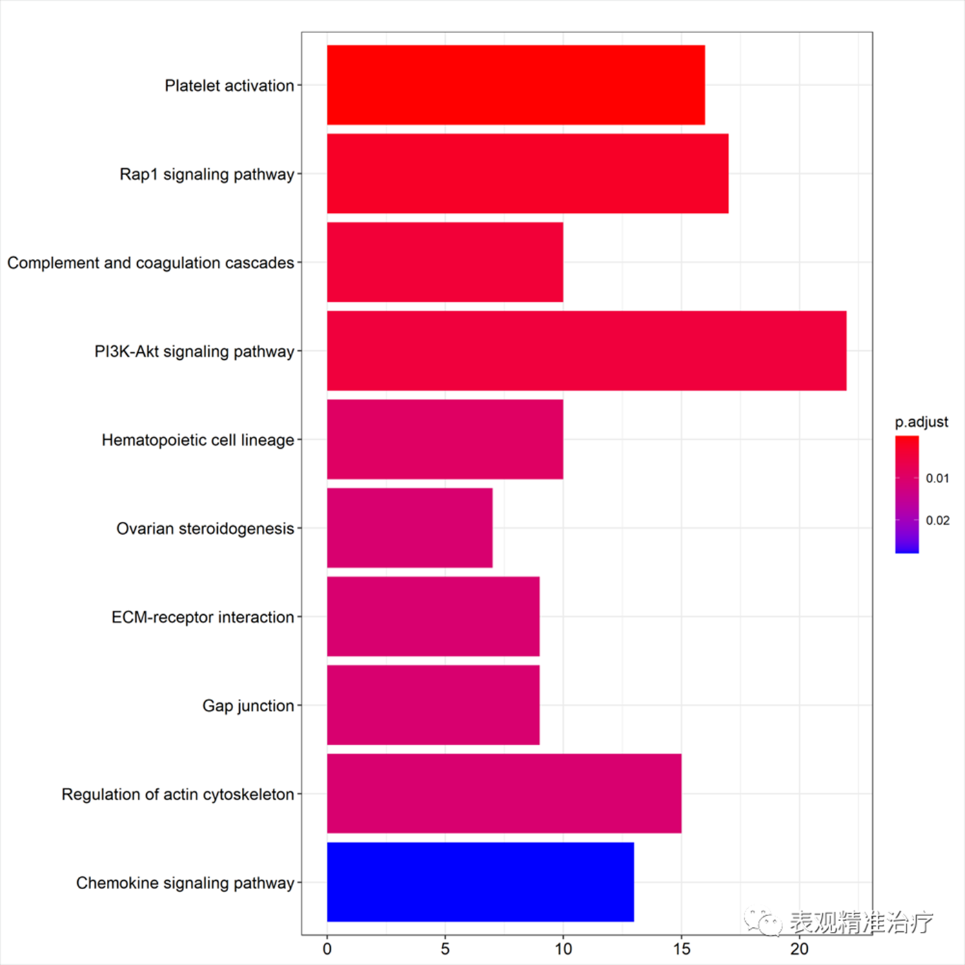
条形图
横轴为基因个数,纵轴为富集到的KEGG Terms的描述信息。颜色对应p.adjust值,红色p值小,蓝色p值大。
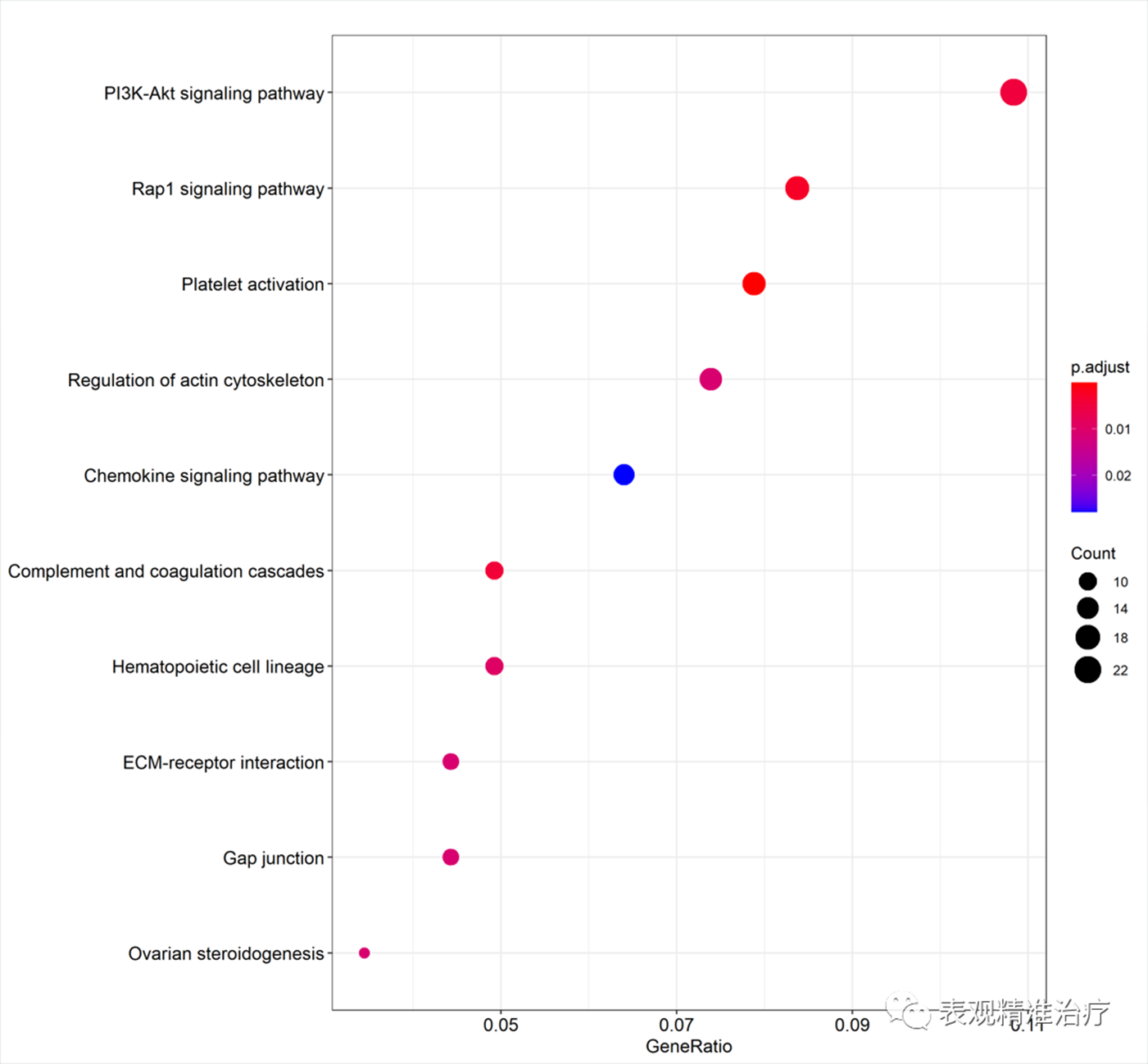
点图
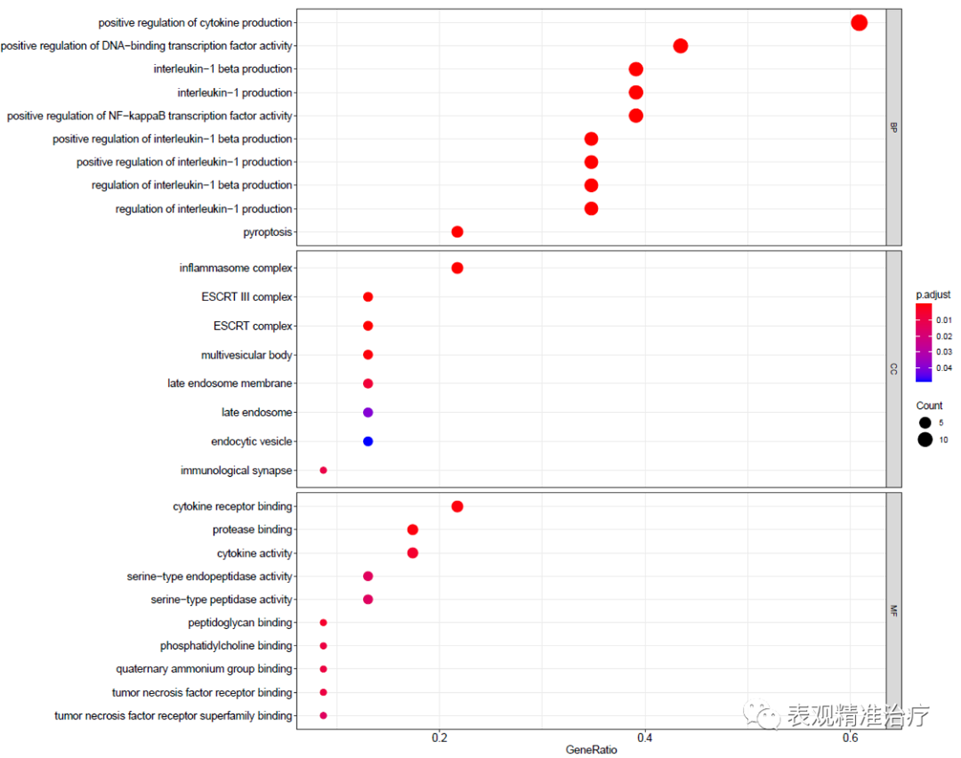
横轴为GeneRatio,代表该KEGG term下富集到的基因个数占列表基因总数的比例。纵轴为富集到的KEGG Terms的描述信息。
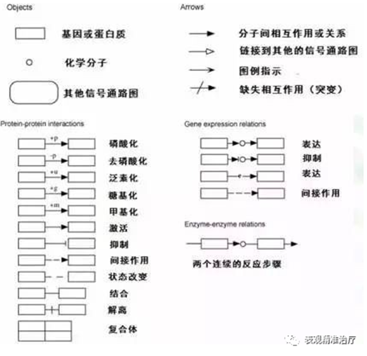
通路图
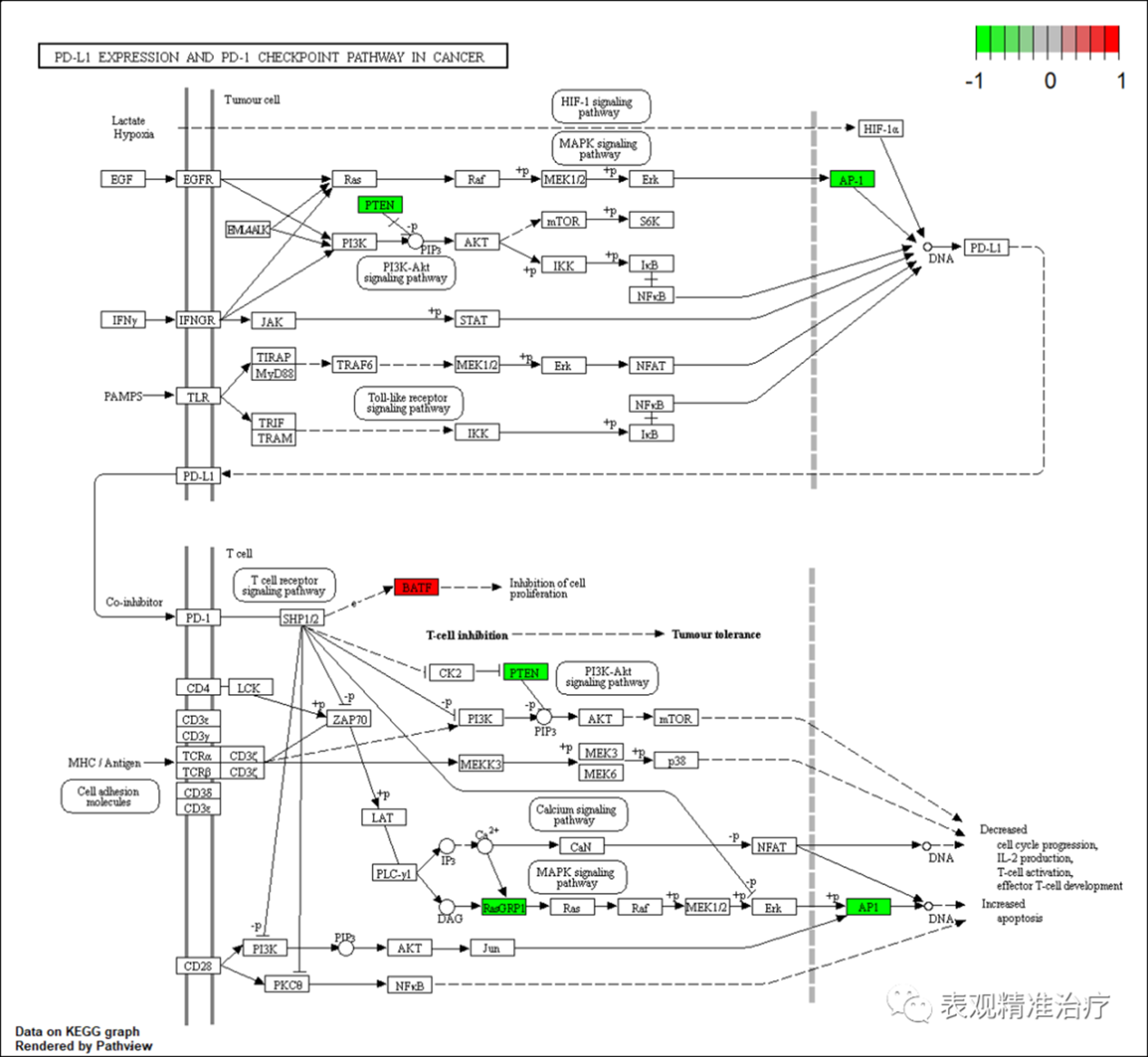
这个通路图可以说是KEGG分析的精华,具体该如何看,详细见下面的图例
GO富集分析
setwd("J:\\Bioinformatics\\R\\76Autophagy\\11.GO")
rt=read.table("id.txt",sep="\t",header=T,check.names=F)
rt=rt[is.na(rt[,"entrezID"])==F,]
gene=rt$entrezID
#GO富集分析
kk <- enrichGO(gene = gene,
OrgDb = org.Hs.eg.db,
pvalueCutoff =0.05,
qvalueCutoff = 0.05,
ont="all",
readable =T)
write.table(kk,file="GO.txt",sep="\t",quote=F,row.names = F) #???渻??????
#绘制条形图
pdf(file="barplot.pdf",width = 15,height = 12)
barplot(kk, drop = TRUE, showCategory =10,split="ONTOLOGY") + facet_grid(ONTOLOGY~., scale='free')
dev.off()
#绘制点图
pdf(file="bubble.pdf",width = 15,height = 12)
dotplot(kk,showCategory = 10,split="ONTOLOGY") + facet_grid(ONTOLOGY~., scale='free')
dev.off()
结果说明
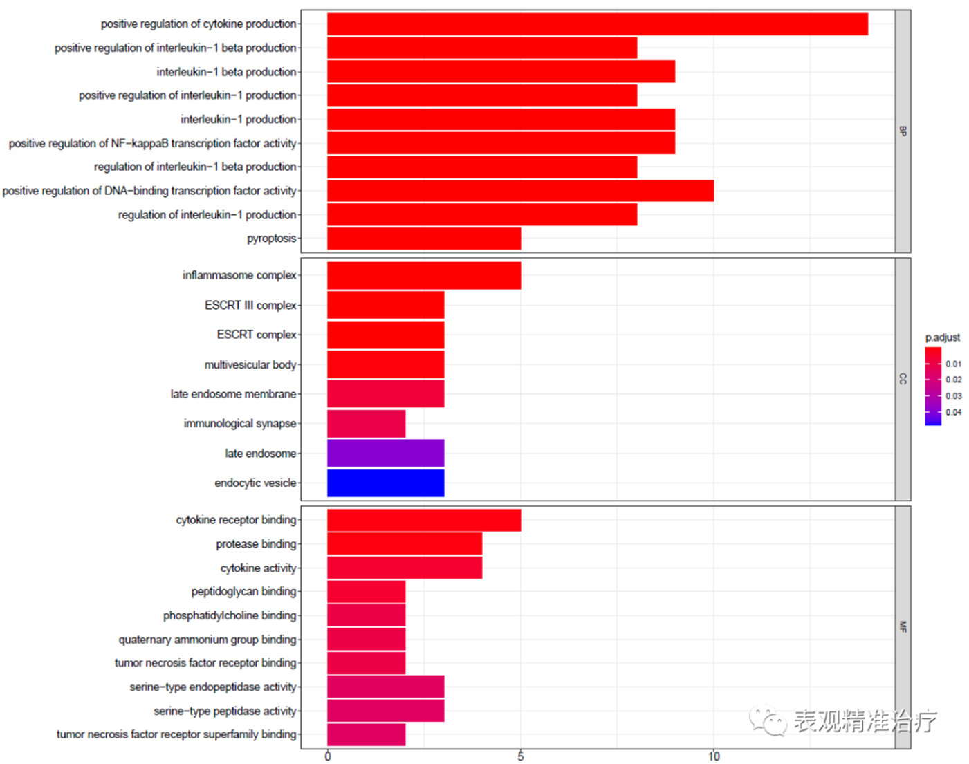
条形图
图例与KEGG相同,只不过针对每一个GO分类进行了分类展示。
点图
此外对于富集分析的可视化形式还有很多,比如GO富集中的有向无环图,GO term的Enrichment Map,热图及upset图等。
图文:张皓旻
本文编辑:李新龙